
1. INTRODUCTION
Pancreatic cancer (PC) is the deadliest disease, ranked 12th with a <5% survival rate among the other cancers. Despite advancements in disease treatments and therapies, the prognosis of PC remains unsatisfactory [1]. To find abnormal expressions in the genes, an efficient differentially expressed genes (DEG) analysis technique is needed. Obesity, smoking, drinking alcohol, and eating meals high in saturated fats are the causes of PC [2]. The advancement in genome molecular profiling provides a way to investigate the structure of tumors at the genome level. Gene expression profiling is the most common approach to molecular profiling and is used to measure the expression levels of a vast number of genes simultaneously. The differential gene expression (DGE) analysis is crucial for identifying the target biomarkers for any disease. This DGE analysis can be done using two popular transcriptomic techniques: microarrays and ribonucleic acid sequencing (RNA-seq).
The microarray technology can identify the DEGs but suffers from a few limitations, such as being unable to identify novel and low-expressed transcripts and having a limited dynamic range [3]. RNA-seq is a next-generation sequencing technique, also called a high-throughput sequencing method, that is adopted in clinical research to synthesize complementary deoxyribonucleic acid (cDNA) transcripts [4]. RNA-seq is often used to identify the expression changes in the gene transcripts under two or more groups (conditions). It has the ability to detect isoforms and novel transcripts. It also has a bigger dynamic range [5,6]. The DEG analysis is essential in cancer research to assess the biological variation in genes and identify gene biomarkers for disease diagnosis and prognosis. There are several bioconductor tools available for DGE analysis of RNA-seq counts data, including Limma [7], EdgeR [8], EBseq [9], and DEseq2 [10]. The pipeline for RNA sequencing data analysis includes the following steps: First, the raw reads are aligned to the reference genome using aligners such as STAR [11] and Bowtie 2 [12]. Next, aligned reads are annotated and summarized. Finally, the gene counts are normalized to reduce the variation of counts among samples. The normalized count data is then further analyzed using any statistical or machine learning (ML) methods for identifying DEGs.
ML is an interdisciplinary field that provides various supervised and unsupervised learning techniques for prediction, feature selection, and classification problems. It plays a key role in multidisciplinary fields like healthcare, business, agriculture, biosciences, etc. [13]. In recent days, ML techniques have been widely used in medical applications [14], bioinformatics studies, including image analysis, cancer research [15,16], and gene biomarker identification [17]. ML and deep learning models can be trained on any size of data, even complex data. These models are also applied to a huge variety of problems in genetics and genomics, such as identifying transcription factor bindings, predicting gene function, and disease phenotypes. [18]. Ensemble learning is an approach to ML in which the insights from multiple models are combined together for better prediction performance. There are three main classes in ensemble learning techniques: bagging, boosting, and stacking.
The objective of the paper is to propose an effective novel ensemble-learning stacking-based classifier model to classify gene expressions from RNA-seq data for PC. The remaining sections of the paper are organized as follows: Section 2 discusses materials, methods used, and methodology; Section 3 shows the results; Section 4 is a discussion about results and critical review analysis; and Section 5 concludes the paper.
2. MATERIALS AND METHODS
This section discusses the dataset, methods used, and methodology followed in our work.
2.1. About the Dataset
The RNA-seq (messenger RNA) data obtained from the Cancer Genome Atlas-Pancreatic Adenocarcinoma (PAAD) project database from the National Cancer Institute Genomic Data Commons portal consists of read counts of 20,532 genes for 178 PAAD samples [19]. As a pre-processing step, we are eliminating the genes whose read counts in the sum of all samples are <10. After this step, the resultant dataset has 19,258 genes and 178 feature samples.
2.2. Methodology
The preprocessed RNA-seq data of size 19,258 × 178 is evaluated for DEGs using edgeR and DESeq2 bioconductor packages in the R language. We set the experimental conditions based on their survival status (alive or deceased) for both tools in DGE analysis. We have collected the DEGs obtained from both tools and constructed a new dataset (D) of 1825 DEGs and 178 features for classification with three target class labels: up (up-regulated), down (downregulated), and NS (not significant). We applied principal component analysis (PCA) as a feature selection technique to identify the principal components (PCs) with high variance [20]. From the PCA results, we have selected the first 15 PCs that show greater than 90% variance in the data. Since the resultant dataset (Dp) is very imbalanced between up and down class labels, we have applied SMOTE to balance each class count [21]. Later, the updated oversampled dataset (Dps) of 2565 genes and 15 feature samples was split into 65% for training and 35% for testing. The stacking CV (SCV) classifier is stacked with K-nearest neighbor (KNN), random forest (RF), gradient boosting (GB), and logistic regression (LR) classifiers. The stack of the first three models acts as a level-1 classifier, and the LR model acts as a level-2 or meta-classifier. We used 10-fold cross-validation, and the hyper-parameters of the models were tuned using the grid search method during the training phase. Finally, the fine-tuned SCV classifier model was tested on the test dataset to evaluate the model’s performance. Figure 1 shows the detailed process of our methodology.
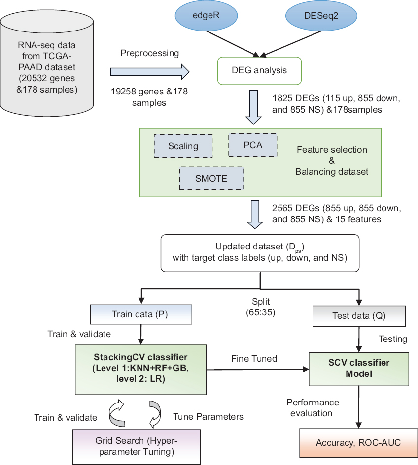 | Figure 1: The detailed flowchart shows methodology of our work. [Click here to view] |
2.3. DEG Analysis
We used two bioconductor package tools called edgeR (Empirical Analysis of Digital Gene Expression in R) and DEseq2 for DEG analysis. The dataset was analyzed using both tools, and the results were intersected to find common DEGs identified by both tools. These tools are open source and available under a general public license from the bioconductor site (http://bioconductor.org).
2.3.1. edgeR
This algorithm computes the dispersion of genes among samples using weighted likelihood and F-test techniques. It can perform a pair-wise comparison between two or more groups or conditions. The edgeR requires two inputs: one is the read count data, and another is the factor that specifies the experimental conditions, cell types, or disease states for each sample. It models the data using a negative binomial distribution, using Equation 1.
 |
Dgi ~ NB (Ripgj, øg)(1)
Here, Ri is the data size, D is the count of gene g in the ith sample, and pgj is the relative abundance of gene g in the jth experimental group to which sample i belongs. øg is the dispersion that shows the biological variation between the samples.
2.3.2. DESeq2
This algorithm also uses the negative binomial distribution, similar to edgeR, and the Wald and likelihood ratio tests for statistical evaluation. The DGE analysis pipeline of this algorithm includes the following steps: estimate size factor, estimate dispersions, fit linear model, and hypothesis testing. DESeq2 performs the DEG analysis based on the read count variation among the samples under the given experimental conditions.
2.4. Ensemble Learning
Ensemble methods use multiple algorithms to build an effective model with better performance than a standalone model. In general, the poor models were assembled to gather the insights of all models. Although these models may require more computation and time, depending on the size of the model, they claim to be more efficient in terms of improving the accuracy of the model. In our work, we used the SCV classifier, which is an extension of the stacking ensemble class and combines multiple classification methods via a meta-classifier [22]. To avoid the overfitting problem with a standard stacking classifier, an SCV classifier is added with cross-validation functionality. The dataset is split into k-folds, and in k subsequent rounds, k-1 folds are used to fit the level-1 classifiers. The predictions of the level-1 classifier in each round were stacked and passed as input to the level-2 classifier (meta-classifier). The detailed steps in the SCV classifier are shown in Figure 2.
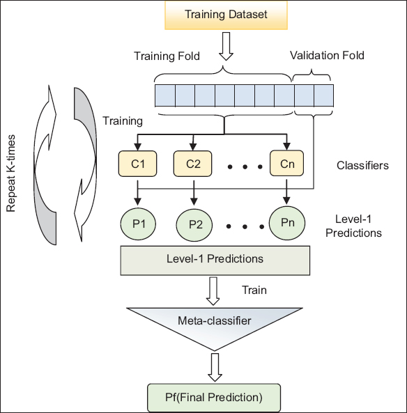 | Figure 2: The working procedure of the stacking CV classifier. [Click here to view] |
2.5. Model Evaluation Metrics
The performance of classification algorithms will be evaluated using metrics such as accuracy, precision, recall, F1-score, and receiver operating characteristics area under the curve (ROC-AUC). A confusion matrix (CM) is a class-wise distribution of the results of the classification model. The typical classes in CM include true positive (TP), false positive (FP), true negative (TN), and false negative (FN). The accuracy of a model is the ratio between correctly classified samples and total samples in the dataset [23]. The accuracy of a model (M) is calculated using Equation 2, given below.

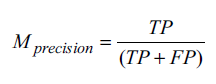
Here, TP is the number of samples predicted correctly as positives, TN is the number of samples predicted correctly as negatives, FP is the number of samples predicted as positive but actually negative, and FN is the number of samples predicted as negative but actually positive. The precision of a model is the ratio between TP and the total number of samples classified as positive, as shown in Equation 3.
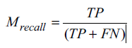
The recall of a model is the ratio between TP and the total number of samples that are actually positive. It is also called sensitivity or true positive rate (TPR), and it is calculated by using Equation 4 shown below.
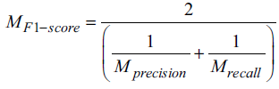
The F1-score of a model provides the combined idea of precision and recall. It is the weighted average of precision and recall. The F1-score is calculated using Equation 5, shown below.
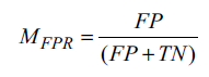
The false positive rate (FPR) of the model is the ratio between FP and the total number of samples that are actually negative. It is calculated using Equation 6, shown below.
ROC-AUC is a measure that captures the model’s distinguishability among the classes. A higher value of the AUC determines better predictions from the model [24]. ROC is plotted between TPR on the Y-axis and FPR on the X-axis. As our problem falls under a multi-class classification, to obtain FPR and TPR, the predicted output should be binarized. This can be done in two ways: the One versus Rest (OvR) method or the One versus One method. In the first method, each class is compared against all other classes. The second way compares every unique pair-wise combination of classes. In our work, we employed the OvR method for binarization.
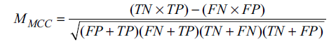
We used Matthew’s correlation coefficient (MCC) for our model evaluation. MCC will measure the quality of the classifications. It can be used for both binary and multiclass classifications [25]. It is the best measure to summarize the confusion matrix. The MCC value of a model is calculated using Equation 7, shown below.
3. RESULTS
3.1. Identification of DEGs
From the statistical computation results of edgeR and DESeq2, based on the log2 fold change (log2FC) and the probability (P) values, the DEGs were identified between the alive and deceased conditions. We set the threshold as log2FC ≥ 1 and P < 0.05 (assuming 5% false discovery rate) for up-regulated genes, log2FC < −1 and P < 0.05 for down-regulated genes, and the rest of the genes were treated as not significant (NS). DESeq2 and edgeR identify a total of 584 (51 up-regulated and 533 down-regulated) and 787 (95 up-regulated and 692 down-regulated), respectively, as DEGs, out of which 401 (31 up-regulated and 370 down-regulated) DEGs are common in both. Tables 1 and 2 show the top ten DEGs along with their statistical values identified by edgeR and DESeq2, respectively.
Table 1: List of top 10 DEGs and their statistical values obtained from edgeR tool.
| S. No. | Gene name | log2 fold change | logCPM | P-value | FDR |
|---|---|---|---|---|---|
| 1. | LY6H | –3.464 | 2.975 | 5.78E-26 | 9.11E-22 |
| 2. | LRRC4B | –2.762 | 2.552 | 1.46E-24 | 1.15E-20 |
| 3. | DRAIC | –3.759 | 1.874 | 4.50E-23 | 2.36E-19 |
| 4. | C1QL1 | –3.521 | 4.084 | 1.12E-22 | 4.42E-19 |
| 5. | SYT5 | –3.704 | 4.061 | 8.23E-22 | 2.59E-18 |
| 6. | SEZ6 | –3.928 | 2.855 | 1.13E-21 | 2.97E-18 |
| 7. | ATP1A3 | –3.073 | 3.452 | 1.88E-21 | 4.23E-18 |
| 8. | HAP1 | –3.262 | 2.785 | 6.13E-21 | 1.21E-17 |
| 9. | AGT | –2.927 | 7.504 | 2.98E-20 | 5.21E-17 |
| 10. | TMEM145 | –3.028 | 1.355 | 4.20E-20 | 6.61E-17 |
DEG: Differentially expressed genes, FDR: False discovery rate
Table 2: List of Top 10 DEGs with their statistical values obtained from DESeq2 tool.
| S. No. | Gene name | Base mean | log2 fold change | lfcSE | stat | P-value | P-adj |
|---|---|---|---|---|---|---|---|
| 1. | RUNDC3A | 381.290 | –2.789 | 0.309 | –9.014 | 1.99E-19 | 3.68E-15 |
| 2. | APLP1 | 1804.481 | –2.493 | 0.282 | –8.832 | 1.03E-18 | 9.54E-15 |
| 3. | LU1 | 263.620 | –1.655 | 0.194 | –8.509 | 1.76E-17 | 7.42E-14 |
| 4. | CYP46A1 | 31.875 | –2.008 | 0.236 | –8.502 | 1.87E-17 | 7.42E-14 |
| 5. | MSI1 | 118.704 | –1.929 | 0.227 | –8.493 | 2.01E-17 | 7.42E-14 |
| 6. | PART 1 | 44.128 | –2.961 | 0.350 | –8.459 | 2.70E-17 | 8.32E-14 |
| 7. | TMEM145 | 36.183 | –2.446 | 0.293 | –8.337 | 7.61E-17 | 1.95E-13 |
| 8. | SPTBN4 | 169.988 | –2.195 | 0.264 | –8.325 | 8.43E-17 | 1.95E-13 |
| 9. | REEP2 | 254.922 | –1.944 | 0.236 | –8.237 | 1.77E-16 | 3.64E-13 |
| 10. | SLC12A5 | 21.305 | –2.284 | 0.279 | –8.176 | 2.94E-16 | 5.44E-13 |
Figure 3a and b show the volcano plots given by DESeq2 and edgeR, respectively. The green, red, and black dots in the plot represent up-regulated, down-regulated, and not-significant genes, respectively. Figure 3c shows the venn diagram that represents the common DEGs between DESeq2 and edgeR results. We merged (union) the up- and down-regulated genes from both results and also added the 855 not significantly expressed genes from both results selected randomly for classification purposes. Finally, the new RNA-seq dataset obtained consists of 1,825 genes (115 up, 855 down, and 855 NS) with read counts for 178 PAAD samples as features and the target variable with 3 classes (up, down, and NS).
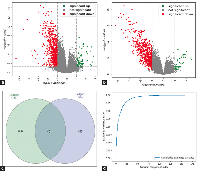 | Figure 3: (a) volcano plot by DESeq2 (b) volcano Plot by edger (c) venn diagram shows common differentially expressed genes between DESeq2 and edgeR results (d) principal component analysis plot explains the relationship between the principal components and their explained variance ratio. [Click here to view] |
3.2. Classification Results
Figure 3d shows the PCA plot between the number of PCs and their explained variance ratio. From the plot, we observe that the first 15 PCs have more than 90% of the explained variance. Table 3 shows the detailed comparison of the performance of various stand-alone ML and other ensemble models with our ensemble SCV classifier. We considered various supervised ML models such as RF, LR, KNN, support vector classifiers (SVC), ensemble models such as GB and extreme gradient boosting (XGB), and a multi-layer perceptron (MLP) model for comparison. The results were shown for three different train-test split categories, and it was observed that our SCV model outperformed in all three categories. The KNN, RF, and GB models are showing the next best performance in terms of accuracy; hence, these models were used as level-1 classifiers in our SCV model. We observed our model performing better with a 65–35 train-test split. The CM (3 × 3) of SCV, KNN, RF, and GB classifiers are shown in Figure 4a-d, respectively. The ROC-AUC curves for SCV, KNN, RF, and GB classifiers are shown in Figure 5a-d, respectively. Each ROC-AUC includes three curves, evaluating each class against other classes using the OvR method. From the figure, our SVC model has the highest area covered under the curve for up versus rest (100%), NS versus rest (98%), and down versus rest (99%).
Table 3: Performance comparison of various stand-alone ML models with SCV classifier.
| S. No. | Model Name | Hyper parameter Information | Train-Test split (%) | Accuracy (%) | Precision | Recall | F1-score |
|---|---|---|---|---|---|---|---|
| 1. | KNN | metric=’euclidean’, n_neighbors=2, weights=’uniform’ | 65–35 | 92 | 93 | 92 | 92 |
| 70–30 | 92 | 93 | 93 | 93 | |||
| 75–25 | 92 | 93 | 93 | 92 | |||
| 2. | RF | random_state=RANDOM_SEED, max_features=’log2’, n_estimators=1000 | 65–35 | 90 | 90 | 90 | 90 |
| 70–30 | 90 | 90 | 90 | 90 | |||
| 75–25 | 90 | 90 | 90 | 90 | |||
| 3 | GB | learning_rate=0.1, max_depth=9, n_estimators=100, subsample=0.5 | 65–35 | 91 | 92 | 91 | 91 |
| 70–30 | 91 | 91 | 91 | 91 | |||
| 75–25 | 90 | 91 | 91 | 90 | |||
| 4. | LR | solver=’lbfgs’, max_iter=400 | 65–35 | 51 | 78 | 50 | 45 |
| 70–30 | 49 | 75 | 48 | 42 | |||
| 75–25 | 48 | 76 | 48 | 42 | |||
| 5. | SVC | C=30, gamma=1, kernel=’rbf’, probability=True | 65–35 | 65 | 80 | 64 | 63 |
| 70–30 | 65 | 79 | 65 | 64 | |||
| 75–25 | 64 | 79 | 64 | 63 | |||
| 6. | XGB | learning_rate=0.2, max_depth=9, n_estimators=50, subsample=0.5 | 65–35 | 90 | 90 | 90 | 90 |
| 70–30 | 90 | 91 | 90 | 90 | |||
| 75–25 | 90 | 90 | 90 | 90 | |||
| 7. | MLP | activation=’relu’, alpha=0.1, hidden_layer_sizes=(10,10,10), learning_rate=’constant’, max_iter=2000, random_state=1000 | 65–35 | 81 | 83 | 81 | 81 |
| 70–30 | 78 | 84 | 78 | 78 | |||
| 75–25 | 84 | 85 | 85 | 84 | |||
| 8. | SCV | shuffle=False, use_probas=True, cv=10, meta_classifier=LR | 65–35 | 96 | 96 | 96 | 96 |
| 70–30 | 94 | 94 | 93 | 93 | |||
| 75–25 | 93 | 92 | 93 | 92 |
ML: Machine learning, KNN: K-nearest neighbour, RF: Random forest, MLP: Multi-layer perceptron, SVC: Support vector classifier, XGB: Extreme gradient boosting, GB: Gradient boosting, LR: Logistic regression, SCV: Stacking CV
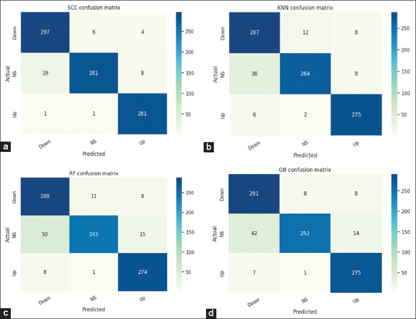 | Figure 4: CM of four classifiers (a) stacking CV (b) K-nearest neighbour (c) random forest (d) gradient boosting. [Click here to view] |
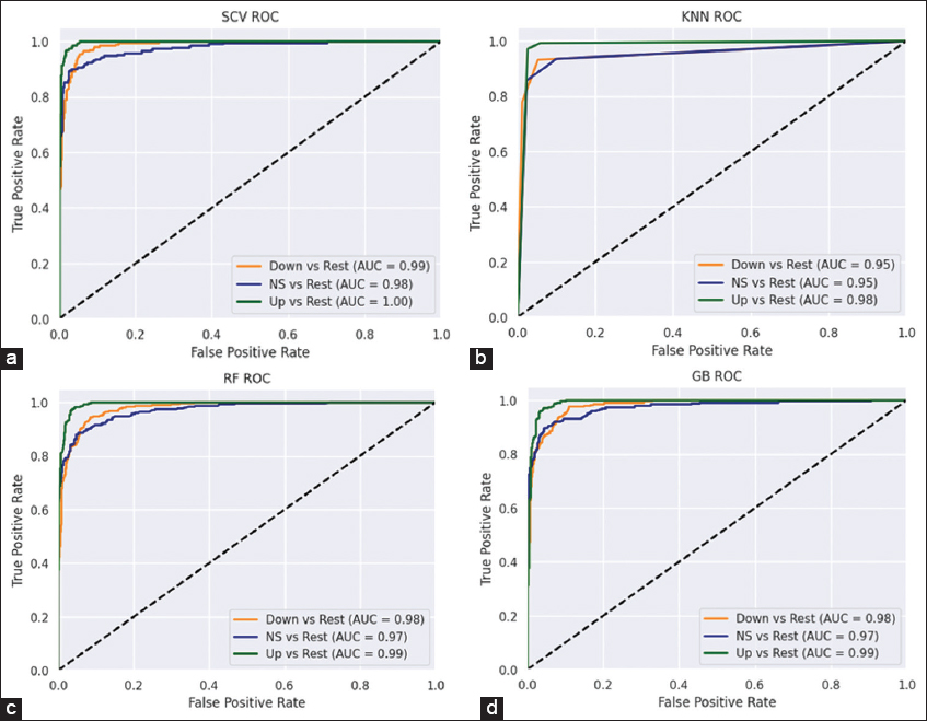 | Figure 5: Receiver operating characteristics-area under the curve of four classifiers (a) stacking CV (b) K-nearest neighbour (c) random forest (d) gradient boosting. [Click here to view] |
Table 4 shows the comparison of the AUC and MCC scores of all the classifiers used in our study. Figure 6 shows the performance comparison in terms of accuracy, ROC, and MCC of our proposed model to the other ML models. From the figure, we can observe that our proposed model has shown a considerable improvement in accuracy, AUC, and MCC scores. It is quite surprising that although the models KNN, XGB, and GB have approximately the same AUC (0.98) as our ensemble model, there is a remarkable difference in their MCC scores.
Table 4: AUC and MCC score comparison of classifiers.
| Model | AUC | Average AUC | MCC | ||
|---|---|---|---|---|---|
| Up versus Rest | Down versus Rest | NS versus Rest | |||
| SCV | 1.00 | 0.99 | 0.98 | 0.99 | 0.92 |
| KNN | 0.98 | 0.95 | 0.95 | 0.96 | 0.88 |
| RF | 0.99 | 0.98 | 0.97 | 0.98 | 0.85 |
| GB | 0.99 | 0.98 | 0.97 | 0.98 | 0.85 |
| MLP | 0.97 | 0.97 | 0.95 | 0.96 | 0.73 |
| SVC | 0.94 | 0.97 | 0.92 | 0.94 | 0.53 |
| XGB | 0.99 | 0.98 | 0.97 | 0.98 | 0.84 |
| LR | 0.93 | 0.94 | 0.88 | 0.91 | 0.35 |
AUC: Area under the curve, MCC: Matthew’s correlation coefficient, KNN: K-nearest neighbour, MLP: Multi-layer perceptron, XGB: Extreme gradient boosting, SVC: Support vector classifier, GB: Gradient boosting, LR: Logistic regression, RF: Random forest, SCV: Stacking CV
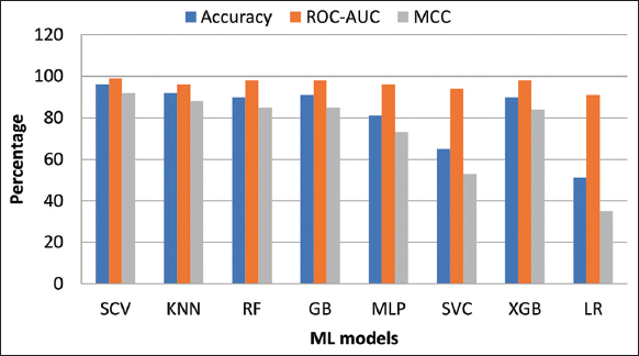 | Figure 6: Performance comparison other machine learning models with our proposed model. [Click here to view] |
4. DISCUSSION
In our work, we have integrated the capabilities of two widely used bioconductor algorithms for DGE analysis, namely edgeR and DESeq2, by combining their respective outputs to create a dataset that is even more useful for classification. Using this result dataset, we built an effective SCV ensemble ML model to classify the DEGs from RNA-seq data on PC. We stacked the three best-performing classifiers at level 1 in the SCV model. We compared the results of our model with those of seven other stand-alone, ensemble ML, and MLP models, and our model performed better in terms of accuracy, recall, precision, F1-score, AUC, and MCC [26]. Our model shows competitively better performance than existing stand-alone models. There is considerable improvement in accuracy and AUC scores among different train-test split ratios. From Tables 1 and 2, we can observe that only one gene (TMEM145) is common in the top 10 DEGs obtained by both algorithms, as they follow different statistical approaches for identifying DEGs. There are only 401 genes that are common in the 1371 DEGs produced by both techniques. Hence, we employed both algorithms for selecting DEGs. Researchers have proposed many ML-based approaches along with the various feature selection methods on both microarray and RNA-seq data of various cancers in the literature. Popular supervised models, like linear support vector machines, KNN, Naive Bayes, Decision Tree (DT), and genetic algorithms for feature selection, were used on lung cancer microarray data classification [27-30].
Chen and Dhahbi [31] have used mixed feature selection methods such as PCA, least absolute shrinkage and selection operator, mRMR, and XGBoost for gene selection from RNA-seq data on lung cancer and applied RF for classification. Zhang and Liu [32] have applied biomarker discovery for hepatocellular carcinoma from high-throughput data using multiple feature selection methods. Yuan et al. [33] have worked on lung cancer gene expression data and used the Monte-Carlo feature selection method. Musheer et al. [34] have worked on different cancer types, such as colon cancer, acute leukemia, prostate tumors, high-grade gliomas, lung cancer II, and leukemia 2 microarray data. They used different gene selection methods, such as independent component analysis and an artificial bee colony-based wrapper approach with Naive Bayes, and the accuracies ranged from 92% to 98%. Pati [35] has classified genes in lung cancer using the Info Gain Ranking Method as a gene feature selection method. The models MLP, sequential minimal optimization, and random subspace were used for classification, and the accuracy ranges from 87% to 92%.
Many of the studies in the literature have used feature selection methods such as genetic algorithms, Recursive feature elimination (RFE), PCA, etc. [36] to identify the target genes from the thousands of gene samples. Certain methods may require a significant amount of time and have been shown to have lower accuracy rates. In our study, we employed the statistical approach for selecting genes under given experimental conditions, and it was very time-effective. The potential of both the DESeq2 and edgeR algorithms enabled the training of our model, which resulted in an effective classifier model. Table 5 shows the critical comparative analysis of the ML models that were proposed in the past in recent literature with our proposed model, related to gene expression classification and their performance.
Table 5: Comparative analysis of the recent ML model’s performance in gene classification.
| Ref | Disease | Dataset and type | Gene selection method | Model (s) and accuracy (%) |
|---|---|---|---|---|
| Rohimat et al., 2022 [27] | Lung cancer | Microarray | Genetic algorithm | Linear SVM (91%) |
| Abdelwahab et al., 2022 [28] | Lung cancer | RNA-seq | RFE | SVM (94%), RF (93%) |
| Coleto-Alcudia and Vega-Rodríguez, 2022 [29] | Cancer | RNA-seq | Filtering and ABCDalgorithm | SVM (93%) |
| Wu et al., 2021 [30] | Breast cancer | RNA-seq | Limma package | KNN (87%), NB (85%), DT (87%), and SVM (90%) |
| Chen and Dhahbi, 2021 [31] | Lung cancer | RNA-seq | Principal component analysis, Lasso, minimal-Redundancy-Maximal relevance (mRMR), and XGboost | RF (90%) |
| This study | Pancreatic cancer | RNA-Seq | edgeR and DESeq2 | Ensemble stacking model with KNN, RF, GB, and LR (96%) |
SVM: Support vector machine, NB: Naive bayes, RNA: Ribonucleic acid, KNN: K-nearest neighbor, RF: Random forest, ML: Machine learning, GB: Gradient boosting, LR: Logistic regression, Lasso: Least absolute shrinkage and selection operator, XGboost: Extreme gradient boosting, ABCD: Artificial bee colony based on dominance
5. CONCLUSION
We proposed a novel ensemble ML model for RNA-seq gene expression classification for PC. We used the edgeR and DESeq2 bioconductor packages for the identification of DEGs and to create a new dataset for classification. Our model learns the genetic signatures from the new dataset. The proposed model has proven to be effective, and it can be used to classify the RNA-seq data for DEG identification in PC. In our subsequent work, we focused on finding the target biomarker genes in PC using our proposed model. We believe that there is a lot of scope for researchers to work on building bio-ML models to analyze different types of omics data.
6. AUTHORS’ CONTRIBUTIONS
All authors made substantial contributions to conception and design, acquisition of data, or analysis and interpretation of data; took part in drafting the article or revising it critically for important intellectual content; agreed to submit to the current journal; gave final approval of the version to be published; and agreed to be accountable for all aspects of the work. All the authors are eligible to be authors as per the International Committee of Medical Journal Editors (ICMJE) requirements and guidelines.
7. FUNDING
There is no funding to report.
8. CONFLICTS OF INTEREST
The authors report no financial or other conflicts of interest in this work.
9. ETHICAL APPROVALS
This study does not involve experiments on animals or human subjects.
10. DATA AVAILABILITY
Available from: https://gdac.broadinstitute.org, https://github.com/GJRao/BioInformatics/blob/main/SCV%20classifier/data_mrna.rar.
11. PUBLISHER’S NOTE
This journal remains neutral with regard to jurisdictional claims in published institutional affiliations.
REFERENCES
1. Lu W, Li N, Liao F. Identification of key genes and pathways in pancreatic cancer gene expression profile by integrative analysis. Genes (Basel) 2019;10:612. [CrossRef]
2. Zhao L, Zhao H, Yan H. Gene expression profiling of 1200 pancreatic ductal adenocarcinoma reveals novel subtypes. BMC Cancer 2018;18:603. [CrossRef]
3. Tarca AL, Romero R, Draghici S. Analysis of microarray experiments of gene expression profiling. Am J Obstet Gynecol 2006;195:373-88. [CrossRef]
4. Turgut S, Da?tekin M, Ensari T. Microarray Breast Cancer Data Classification Using Machine Learning Methods. In:2018 Electric Electronics, Computer Science, Biomedical Engineerings'Meeting (EBBT). Istanbul, Turkey:IEEE;2018. 1-3. [CrossRef]
5. Stark R, Grzelak M, Hadfield J. RNA sequencing:The teenage years. Nat Rev Genet 2019;20:631-56. [CrossRef]
6. Aguiar D, Cheng LF, Dumitrascu B, Mordelet F, Pai AA, Engelhardt BE. Bayesian nonparametric discovery of isoforms and individual specific quantification. Nat Commun 2018;9:1681. [CrossRef]
7. Smyth GK. Limma:Linear models for microarray data. In:Bioinformatics and Computational Biology Solutions using R and Bioconductor. New York:Springer New York;2005. 397-420. [CrossRef]
8. Robinson MD, McCarthy DJ, Smyth GK. edgeR:A bioconductor package for differential expression analysis of digital gene expression data. Bioinformatics 2010;26:139-40. [CrossRef]
9. Leng N, Dawson JA, Thomson JA, Ruotti V, Rissman AI, Smits BM, et al. EBSeq:An empirical Bayes hierarchical model for inference in RNA-seq experiments. Bioinformatics 2013;29:1035-43. [CrossRef]
10. Love MI, Huber W, Anders S. Moderated estimation of fold change and dispersion for RNA-seq data with DESeq2. Genome Biol 2014;15:550. [CrossRef]
11. Dobin A, Davis CA, Schlesinger F, Drenkow J, Zaleski C, Jha S, et al. STAR:Ultrafast universal RNA-seq aligner. Bioinformatics 2013;29:15-21. [CrossRef]
12. Langmead B, Salzberg SL. Fast gapped-read alignment with Bowtie 2. Nat Methods 2012;9:357-9. [CrossRef]
13. Wang L, Xi Y, Sung S, Qiao H. RNA-seq assistant:Machine learning based methods to identify more transcriptional regulated genes. BMC Genomics 2018;19:546. [CrossRef]
14. Shehab M, Abualigah L, Shambour Q, Abu-Hashem MA, Shambour MK, Alsalibi AI, et al. Machine learning in medical applications:A review of state-of-the-art methods. Comput Biol Med 2022;145:105458. [CrossRef]
15. Stupnikov A, McInerney CE, Savage KI, McIntosh SA, Emmert-Streib F, Kennedy R, et al. Robustness of differential gene expression analysis of RNA-seq. Comput Struct Biotechnol J 2021;19:3470-81. [CrossRef]
16. Alharbi F, Vakanski A. Machine learning methods for cancer classification using gene expression data:A review. Bioengineering (Basel) 2023;10:173. [CrossRef]
17. Li R, Zhu J, Zhong WD, Jia Z. Comprehensive evaluation of machine learning models and gene expression signatures for prostate cancer prognosis using large population cohorts. Cancer Res 2022;82:1832-43. [CrossRef]
18. Azzawi H, Hou J, Alnnni R, Xiang Y. SBC:A New Strategy for Multiclass Lung Cancer Classification Based on Tumour Structural Information and Microarray Data. In:2018 IEEE/ACIS 17th International Conference on Computer and Information Science (ICIS). Singapore:IEEE;2018. 68-73. [CrossRef]
19. Broad GDAC Firehose;(n.d.). Available from:https://gdac.broadinstitute.org [Last accessed on 2023 May 20].
20. Jolliffe I. Principal component analysis. In:Lovric M, editor. International Encyclopedia of Statistical Science. Berlin, Heidelberg:Springer;2011. [CrossRef]
21. Chawla NV, Bowyer KW, Hall LO, Kegelmeyer WP. SMOTE:Synthetic minority over-sampling technique. J Artif Intell Res 2002;16:321-57. [CrossRef]
22. Michailidis M. StackNet, StackNet Meta Modelling Framework;2017. Available from:https://github.com/kaz-anova/stacknet [Last accessed on 2023 Jun 15].
23. Stehman SV. Selecting and interpreting measures of thematic classification accuracy. Remote Sens Environ 1997;62:77-89. [CrossRef]
24. Fawcett T. An introduction to ROC analysis. Pattern Recognit Lett 2006;27:861-74. [CrossRef]
25. Matthews BW. Comparison of the predicted and observed secondary structure of T4 phage lysozyme. Biochim Biophys Acta 1975;405:442-51. [CrossRef]
26. Jagadeeswara Rao G, Siva Prasad A, Sai Srinivas S, Sivaparvathi K, Panda N. Data classification by ensemble methods in machine learning. In:Mohanty MN, Das S, editors. Advances in Intelligent Computing and Communication. Lecture Notes in Networks and Systems. Vol. 430. Singapore:Springer;2022. [CrossRef]
27. Rohimat TN, Nhita F, Kurniawan I. Implementation of Genetic Algorithm-Support Vector Machine on Gene Expression Data in Identification of Non-Small Cell Lung Cancer in Nonsmoking Female. In:2022 5th International Conference of Computer and Informatics Engineering (IC2IE). Jakarta, Indonesia:IEEE;2022. 361-6.
28. Abdelwahab O, Awad N, Elserafy M, Badr E. A feature selection-based framework to identify biomarkers for cancer diagnosis:A focus on lung adenocarcinoma. PLoS One 2022;17:e0269126. [CrossRef]
29. Coleto-Alcudia V, Vega-Rodríguez MA. A multi-objective optimization approach for the identification of cancer biomarkers from RNA-seq data. Expert Syst Appl 2022;193:116480. [CrossRef]
30. Wu J, Hicks C. Breast cancer type classification using machine learning. J Pers Med 2021;11:61. [CrossRef]
31. Chen JW, Dhahbi J. Lung adenocarcinoma and lung squamous cell carcinoma cancer classification, biomarker identification, and gene expression analysis using overlapping feature selection methods. Sci Rep 2021;11:13323. [CrossRef]
32. Zhang Z, Liu ZP. Robust biomarker discovery for hepatocellular carcinoma from high-throughput data by multiple feature selection methods. BMC Med Genomics 2021;14:112. [CrossRef]
33. Yuan F, Lu L, Zou Q. Analysis of gene expression profiles of lung cancer subtypes with machine learning algorithms. Biochim Biophys Acta Mol Basis Dis 2020;1866:165822. [CrossRef]
34. Musheer RA, Verma CK, Srivastava N. Novel machine learning approach for classification of high-dimensional microarray data. Soft Comput 2019;23:13409-21. [CrossRef]
35. Pati J. Gene expression analysis for early lung cancer prediction using machine learning techniques:An eco-genomics approach. IEEE Access 2018;7:4232-8. [CrossRef]
36. Xu J, Wu P, Chen Y, Zhang L. Comparison of Different Classification Methods for Breast Cancer Subtypes Prediction. In:Proceedings International Conference on Security, Pattern Analysis, and Cybernetics (SPAC);2018. p. 91-6. [CrossRef]